Time Weighted Average and Value in Azure Data Explorer

This article is contributed. See the original author and article here.

Azure Data Explorer (ADX) supports time series aggregation at scale, either by the summarize operator that keeps the aggregated data in tabular format or by the make-series operator that transforms it to a set of dynamic arrays. There are multiple aggregation functions, out of them avg() is one of the most popular. ADX calculates it by grouping the samples into fixed time bins and applying simple average of all samples inside each time bin, regardless of their specific location inside the bin. This is the standard time bin aggregation as done by SQL and other databases. However, there are scenarios where simple average doesn’t accurately represent the time bin value. For example, IoT devices sending data commonly emits metric values in an asynchronous way, only upon change, to conserve bandwidth. In that case we need to calculate Time Weighted Average (TWA), taking into consideration the exact timestamp and duration of each value inside the time bin. ADX doesn’t have native aggregation functions to calculate time weighted average, still we have just added few User Defined Functions, part of the Functions Library, supporting it:

• time_weighted_val_fl() – Calculates the time weighted value of a metric using linear interpolation.


• time_weighted_avg_fl() – Calculates the time weighted average of a metric using fill forward interpolation.


• time_weighted_avg2_fl() – Calculates the time weighted average of a metric using linear interpolation.

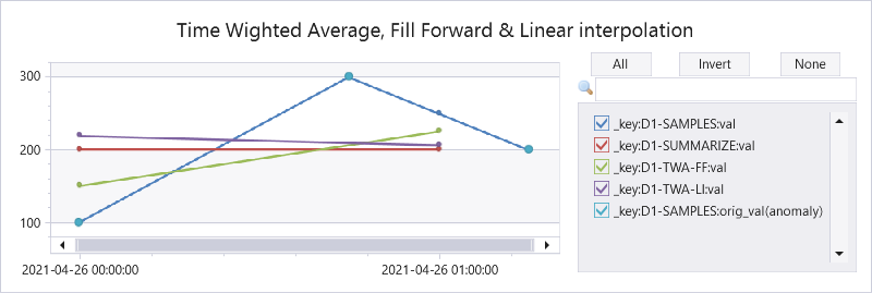
Here is a query comparing the original & interpolated values, standard average by the summarize operator, twa using fill forward and twa using linear interpolation:

let tbl = datatable(ts:datetime,  val:real, key:string) [
    datetime(2021-04-26 00:00), 100, 'D1',
    datetime(2021-04-26 00:45), 300, 'D1',
    datetime(2021-04-26 01:15), 200, 'D1',
];
let stime=datetime(2021-04-26 00:00);
let etime=datetime(2021-04-26 01:15);
let dt = 1h;
//
tbl
| where ts between (stime..etime)
| summarize val=avg(val) by bin(ts, dt), key
| project-rename _ts=ts, _key=key
| extend orig_val=0
| extend _key = strcat(_key, '-SUMMARIZE'), orig_val=0
| union (tbl
| invoke time_weighted_val_fl('ts', 'val', 'key', stime, etime, dt)
| project-rename val = _twa_val
| extend _key = strcat(_key, '-SAMPLES'))
| union (tbl
| invoke time_weighted_avg_fl('ts', 'val', 'key', stime, etime, dt)
| project-rename val = tw_avg
| extend _key = strcat(_key, '-TWA-FF'), orig_val=0)
| union (tbl
| invoke time_weighted_avg2_fl('ts', 'val', 'key', stime, etime, dt)
| project-rename val = tw_avg
| extend _key = strcat(_key, '-TWA-LI'), orig_val=0)
| order by _key asc, _ts asc
// use anomalychart just to show original data points as bold dots
| render anomalychart with (anomalycolumns=orig_val, title='Time Wighted Average, Fill Forward & Linear interpolation')

Explaining the results:

Note that all functions work on multiple time series, partitioned by supplied key.

You are welcome to try these functions and share your feedback!

Brought to you by Dr. Ware, Microsoft Office 365 Silver Partner, Charleston SC.